Introduction to R

Nithin M

Aug 28, 2025

About Me

Nithin M

Doctoral Student, Economics

Indian Institute of Technology Kharagpur

@nithin_eco @nithinmkp [ write2nithinm@gmail.com]

About You

• R enthusiasts
• Economics students (Most probably)
• Practitioners

Basics of R (RStudio IDE)

Outline

Basics of R (RStudio IDE)

Data Analysis

Regression Analysis

Why R

Pros

• R is Free
• language for Data science (Python too)
• Written with statisticians in mind
• Vectorised language
• Most up to date econometric techniques

Cons

• steep learning curve
• speed (compared to Julia, C)

Software installation

1. Download R.

2. Download RStudio.

Live Demo

R-Console

• Version , name
• License
• prompt

Basic arithmetic

R- a powerful caclulator

1+2 ## Addition

[1] 3

6-7 ## Subtraction

[1] -1

5/2 ## Division

[1] 2.5

2^3 ## Exponentiation

[1] 8

2+4*1^3 ## Standard order of precedence (`*` before `+`, etc.)

[1] 6

Basic arithmetic (cont.)

100 %/% 60 #<1> integer division

[1] 1

100 %% 60 #<2> moduluo operator/remainder

[1] 40

Logical Operations and Booleans

• logical operations always result in booleans (TRUE,FALSE)
• ‘&’, ‘|’ and ‘!’
• order of preference : ‘logical’ > ‘boolean’
• another uncommon logical operator is %in%

1 > 2

[1] FALSE

1 > 2 & 1 > 0.5 ## The "&" stands for "and"

[1] FALSE

1 > 2 | 1 > 0.5 ## The "|" stands for "or" 

[1] TRUE

4 %in% 1:10

[1] TRUE

# 2 = 3 ## This will cause an error
2 == 3 # This will run

[1] FALSE

Question

1 > 0.5 & 2

[1] TRUE

1 > 0.5 & 1 > 2

[1] FALSE

0.1 + 0.2 == 0.3

[1] FALSE

But we need an IDE

• code editing
• syntax higlighting
• convinence

Enter RStudio

Intro to Programming

• writing a set of instructions
• fixed rules
• elements of style

If you will be doing computational work there are:

• Language-independent coding basics you should know
  • Arrays are stored in memory in particular ways
• Language-independent best practices you should use
  • Indent to convey program structure (or function in Python)
• Language-dependent idiosyncracies that matter for function, speed, etc
  • Julia: type stability; R: vectorize

Intro to programming (Contd..)

Learning these early will:

• Make coding a lot easier
• Reduce total programmer time
• Reduce total computer time
• Make your code understandable by someone else or your future self
• Make your code flexible

Some R basics (OOP in R)

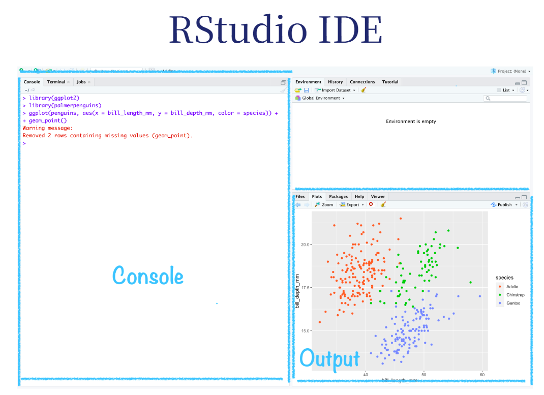
1. Everything is an object.

2. Everything has a name.

3. You do things using functions.

plot(1:4, seq(2,8,by=2),type="l")

4. Functions come pre-written in packages (i.e. “libraries”), although you can — and should — write your own functions too.

OOP in R

• Types of Objetcs
  • data types
  • classes
• Not full OOP as in C (trade off ??)

Common Objects in R

• Vectors
• Matrices
• Data frames
• functions
• lists

Data Types

• In R everything is a vector
• Atomic Vectors: Character, Numeric(double, int), Logical, Complex, Raw
• Vectors are homogenous collection of items
• Matrices are rectangular representations of homogenous items
• Dataframes are enhanced matrices, can contain items of different type
• lists can include anything

Vectors

• you can create a vector of say marks in 5 subjects

marks <- c(56,89,67,98,99) # c() is the concatenation operator
marks

[1] 56 89 67 98 99

• but there is a problem!! which mark refers to which subject??
• solution - named vector (dictionary in python)

names(marks) <- c("maths","english","science","hindi","computer science")
marks

           maths          english          science            hindi 
              56               89               67               98 
computer science 
              99 

• indexing and slicing of vectors

marks[1] # Select first element

maths 
   56 

marks[c(1,4)] # Select 1st and 4th element

maths hindi 
   56    98 

marks["english"] # select using names

english 
     89 

marks[marks >75] # select using logical conditions

         english            hindi computer science 
              89               98               99 

marks[-1] # select everything excludig first one

         english          science            hindi computer science 
              89               67               98               99 

mention python difference here in indexing

What if we now need to store marks of multiple students?? We can use matrices we can create a matrix using matrix function

mat_a <- matrix(c(1,4,57,4,67,78))
mat_a

     [,1]
[1,]    1
[2,]    4
[3,]   57
[4,]    4
[5,]   67
[6,]   78

# check for help
# change number of rows
# use byrow argument
colnames(mat_a) <- "english"
rownames(mat_a) <- letters[1:6]
mat_a

  english
a       1
b       4
c      57
d       4
e      67
f      78

speak about matrix operatiosn, sliding, selection etc too

Exercise

01:15

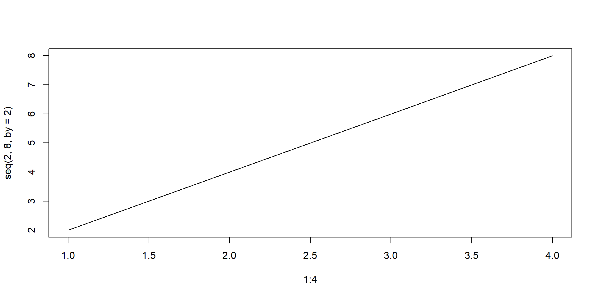
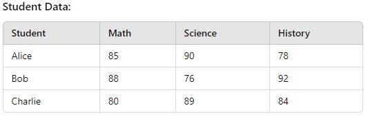
Create a matrix in R that presents data as shown

# Student names
students <- c("Alice", "Bob", "Charlie")

# Marks matrix
marks <- matrix(
  c(85, 90, 78,   # Marks for Alice
    88, 76, 92,   # Marks for Bob
    80, 89, 84),  # Marks for Charlie
  nrow = 3,
  byrow = TRUE
)

# Assigning row and column names
rownames(marks) <- students
colnames(marks) <- c("Math", "Science", "History")

# Display the matrix
marks

        Math Science History
Alice     85      90      78
Bob       88      76      92
Charlie   80      89      84

Consider now we need to add other details of the students like DOB, Adress etc !!

• Matrices cannot do this !! why??
• Solution - Dataframes
• we can create dataframe using data.frame command’ just like matrix command

names <- c("ron", "harry", "irene")
english_marks <- c(56,78,89)
maths_marks <- c(45,98,79)
dob <- c("29/12/1994", "08/11/1991", "24/06/1991")
data.frame(names,english_marks,maths_marks,dob)

  names english_marks maths_marks        dob
1   ron            56          45 29/12/1994
2 harry            78          98 08/11/1991
3 irene            89          79 24/06/1991

talk again about slicing, naming, selection of items in dataframes

Lists

• Can contain anything
• neat way of organising many information

$class1
  names english_marks maths_marks        dob
1   ron            56          45 29/12/1994
2 harry            78          98 08/11/1991
3 irene            89          79 24/06/1991

$class2
  names english_marks maths_marks        dob
1   ron            56          45 29/12/1994
2 harry            78          98 08/11/1991
3 irene            89          79 24/06/1991

Functions

• reuse code

my_func = 
  function(ARGUMENTS) {
    OPERATIONS
    return(VALUE)
  }

• R
• Python

square =        ## Our function name
  function(x) { ## The argument(s) that our function take as an input
    x^2         ## The operation(s) that our function performs
  }
square(4)

[1] 16

def square(x):
   return x**2

square(4)

16

• by default,function returns the last value (not in case of python)
• explicit use of return statements for finer control

Live Demo

Flow of Control

• how statements and operations are evaluated in a function

1. The if statement

if(expression){
    statement
}

Exercise

01:15

Write a function that takes a input and checks if it is a number. If not number, convert to number and caclulate square of the number

check_function <- function(input){
    
    if(is.numeric(input)==FALSE){
        input = as.numeric(input)
    }
    input^2
}
check_function("4")

[1] 16

Flow of Control (Contd..)

2. The else condition

if(expression){
    statement
} else {
  statement
}

3. break Statement
4. next Statement

Exercise

01:15

Write a function that takes a number and prints “odd” or “even”

odd_even <- function(input) {
  if (input %% 2 == 0) {  # Using %% to check even/odd
    print("Even")
  } else {
    print("Odd")
  }
}

odd_even(4)

[1] "Even"

Iteration

Loops

1 for loop

• one of the most important skill
• easiest to use
• entry controlled

for(condtion){
 statement
}

numbers <- seq(1,10)
for(i in numbers){
  print(i^2)
}

[1] 1
[1] 4
[1] 9
[1] 16
[1] 25
[1] 36
[1] 49
[1] 64
[1] 81
[1] 100

2 while loop

• can run infinitely
• exit controlled loop

while(condtion){
 statement
}

i=1
while(i <=100){
  if(i %%10 ==0){
     print(i)
  }
  i = i+1
}

[1] 10
[1] 20
[1] 30
[1] 40
[1] 50
[1] 60
[1] 70
[1] 80
[1] 90
[1] 100

Vectorisation

• Remember I told you R is vectorised language??
• apply a function to every element of a vector at once

• R
• Python

numbers <- 1:20
squares <- numbers^2
squares

 [1]   1   4   9  16  25  36  49  64  81 100 121 144 169 196 225 256 289 324 361
[20] 400

numbers = range(1,21)
numbers**2

TypeError: unsupported operand type(s) for ** or pow(): 'range' and 'int'

import numpy as np
numbers = range(1,21)
numbers = np.array(numbers)
numbers**2

array([  1,   4,   9,  16,  25,  36,  49,  64,  81, 100, 121, 144, 169,
       196, 225, 256, 289, 324, 361, 400])

Packages

• An R package is a collection of functions, data, and documentation that extends the capabilities of base R.
• As on Aug 28, 2025 , There are 22591 packages available in CRAN
• Packages need to be loaded at the start of every ‘new’ session
  • “Base” R comes with tons of useful in-built functions. It also provides all the tools necessary for you to write your own functions.

  • However, many of R’s best data science functions and tools come from external packages written by other users.

Live Demo

Questions

Data Analysis

Outline

Basics of R (RStudio IDE)

Data Analysis

Regression Analysis

Importing the Data

• 2 ways to import an external data

Code

library(readxl) # Readl excel data
library(readr) # Readr csv,text 
library(foreign)
library(haven)  # both to read SPSS, Stata and SAS files

speak about relative paths here, use of here package etc

Data Wrangling

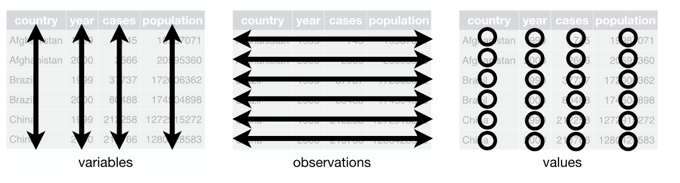
Process of data exploration, manipulation and and transforming data to obtain meaningful information - tidy data - basic operations inlcude sorting, filtering,arranging and calculation of summary statistics

tidy data

• many of the time we need datframes for our analysis.
• we have special forms of dataframes too like tibble, data.table, tsible etc
• these forms depend on R frameworks like base R, tidyverse etc

Selection

• one of the most important operations
• we will use the mtcars datset

                   mpg cyl disp  hp drat    wt  qsec vs am gear carb
Mazda RX4         21.0   6  160 110 3.90 2.620 16.46  0  1    4    4
Mazda RX4 Wag     21.0   6  160 110 3.90 2.875 17.02  0  1    4    4
Datsun 710        22.8   4  108  93 3.85 2.320 18.61  1  1    4    1
Hornet 4 Drive    21.4   6  258 110 3.08 3.215 19.44  1  0    3    1
Hornet Sportabout 18.7   8  360 175 3.15 3.440 17.02  0  0    3    2
Valiant           18.1   6  225 105 2.76 3.460 20.22  1  0    3    1

• we will select only mpg,cyl,and gear column

• Base- R
• Tidyverse

head(mtcars[,c("mpg","cyl","gear")]) # by name

                   mpg cyl gear
Mazda RX4         21.0   6    4
Mazda RX4 Wag     21.0   6    4
Datsun 710        22.8   4    4
Hornet 4 Drive    21.4   6    3
Hornet Sportabout 18.7   8    3
Valiant           18.1   6    3

head(mtcars[,c(1,2,5)]) # by position

                   mpg cyl drat
Mazda RX4         21.0   6 3.90
Mazda RX4 Wag     21.0   6 3.90
Datsun 710        22.8   4 3.85
Hornet 4 Drive    21.4   6 3.08
Hornet Sportabout 18.7   8 3.15
Valiant           18.1   6 2.76

head(mtcars[, grep("^c", names(mtcars))]) # pattern

                  cyl carb
Mazda RX4           6    4
Mazda RX4 Wag       6    4
Datsun 710          4    1
Hornet 4 Drive      6    1
Hornet Sportabout   8    2
Valiant             6    1

head(select(mtcars,c(cyl,mpg,gear)))

                  cyl  mpg gear
Mazda RX4           6 21.0    4
Mazda RX4 Wag       6 21.0    4
Datsun 710          4 22.8    4
Hornet 4 Drive      6 21.4    3
Hornet Sportabout   8 18.7    3
Valiant             6 18.1    3

head(select(mtcars,c(1,2,5)))

                   mpg cyl drat
Mazda RX4         21.0   6 3.90
Mazda RX4 Wag     21.0   6 3.90
Datsun 710        22.8   4 3.85
Hornet 4 Drive    21.4   6 3.08
Hornet Sportabout 18.7   8 3.15
Valiant           18.1   6 2.76

head(select(mtcars,starts_with("c")))

                  cyl carb
Mazda RX4           6    4
Mazda RX4 Wag       6    4
Datsun 710          4    1
Hornet 4 Drive      6    1
Hornet Sportabout   8    2
Valiant             6    1

• cool feature in tidyverse

mtcars |> 
  select(starts_with("c")) |>
  head()

                  cyl carb
Mazda RX4           6    4
Mazda RX4 Wag       6    4
Datsun 710          4    1
Hornet 4 Drive      6    1
Hornet Sportabout   8    2
Valiant             6    1

filtering

subset rows based on conditions

• Base- R
• Tidyverse

head(mtcars[mtcars$cyl == 4 , ] ) # select all cars with 4 cylinders

                mpg cyl  disp hp drat    wt  qsec vs am gear carb
Datsun 710     22.8   4 108.0 93 3.85 2.320 18.61  1  1    4    1
Merc 240D      24.4   4 146.7 62 3.69 3.190 20.00  1  0    4    2
Merc 230       22.8   4 140.8 95 3.92 3.150 22.90  1  0    4    2
Fiat 128       32.4   4  78.7 66 4.08 2.200 19.47  1  1    4    1
Honda Civic    30.4   4  75.7 52 4.93 1.615 18.52  1  1    4    2
Toyota Corolla 33.9   4  71.1 65 4.22 1.835 19.90  1  1    4    1

head(mtcars[mtcars$cyl == 4 | mtcars$gear == 4 , ]) # 4 cylinders or 4 gears

               mpg cyl  disp  hp drat    wt  qsec vs am gear carb
Mazda RX4     21.0   6 160.0 110 3.90 2.620 16.46  0  1    4    4
Mazda RX4 Wag 21.0   6 160.0 110 3.90 2.875 17.02  0  1    4    4
Datsun 710    22.8   4 108.0  93 3.85 2.320 18.61  1  1    4    1
Merc 240D     24.4   4 146.7  62 3.69 3.190 20.00  1  0    4    2
Merc 230      22.8   4 140.8  95 3.92 3.150 22.90  1  0    4    2
Merc 280      19.2   6 167.6 123 3.92 3.440 18.30  1  0    4    4

head(subset(mtcars,mtcars$cyl ==4 ))

                mpg cyl  disp hp drat    wt  qsec vs am gear carb
Datsun 710     22.8   4 108.0 93 3.85 2.320 18.61  1  1    4    1
Merc 240D      24.4   4 146.7 62 3.69 3.190 20.00  1  0    4    2
Merc 230       22.8   4 140.8 95 3.92 3.150 22.90  1  0    4    2
Fiat 128       32.4   4  78.7 66 4.08 2.200 19.47  1  1    4    1
Honda Civic    30.4   4  75.7 52 4.93 1.615 18.52  1  1    4    2
Toyota Corolla 33.9   4  71.1 65 4.22 1.835 19.90  1  1    4    1

mtcars |>
filter(cyl == 4) |>
head()

                mpg cyl  disp hp drat    wt  qsec vs am gear carb
Datsun 710     22.8   4 108.0 93 3.85 2.320 18.61  1  1    4    1
Merc 240D      24.4   4 146.7 62 3.69 3.190 20.00  1  0    4    2
Merc 230       22.8   4 140.8 95 3.92 3.150 22.90  1  0    4    2
Fiat 128       32.4   4  78.7 66 4.08 2.200 19.47  1  1    4    1
Honda Civic    30.4   4  75.7 52 4.93 1.615 18.52  1  1    4    2
Toyota Corolla 33.9   4  71.1 65 4.22 1.835 19.90  1  1    4    1

Sorting

• Base- R
• Tidyverse

head(mtcars[order(mtcars$cyl),]) # sort data by cyl

                mpg cyl  disp hp drat    wt  qsec vs am gear carb
Datsun 710     22.8   4 108.0 93 3.85 2.320 18.61  1  1    4    1
Merc 240D      24.4   4 146.7 62 3.69 3.190 20.00  1  0    4    2
Merc 230       22.8   4 140.8 95 3.92 3.150 22.90  1  0    4    2
Fiat 128       32.4   4  78.7 66 4.08 2.200 19.47  1  1    4    1
Honda Civic    30.4   4  75.7 52 4.93 1.615 18.52  1  1    4    2
Toyota Corolla 33.9   4  71.1 65 4.22 1.835 19.90  1  1    4    1

head(mtcars[order(mtcars$mpg,rev(mtcars$cyl)),])

                     mpg cyl disp  hp drat    wt  qsec vs am gear carb
Cadillac Fleetwood  10.4   8  472 205 2.93 5.250 17.98  0  0    3    4
Lincoln Continental 10.4   8  460 215 3.00 5.424 17.82  0  0    3    4
Camaro Z28          13.3   8  350 245 3.73 3.840 15.41  0  0    3    4
Duster 360          14.3   8  360 245 3.21 3.570 15.84  0  0    3    4
Chrysler Imperial   14.7   8  440 230 3.23 5.345 17.42  0  0    3    4
Maserati Bora       15.0   8  301 335 3.54 3.570 14.60  0  1    5    8

library(tidyverse)
head(arrange(mtcars,cyl)) # sort data by cyl

                mpg cyl  disp hp drat    wt  qsec vs am gear carb
Datsun 710     22.8   4 108.0 93 3.85 2.320 18.61  1  1    4    1
Merc 240D      24.4   4 146.7 62 3.69 3.190 20.00  1  0    4    2
Merc 230       22.8   4 140.8 95 3.92 3.150 22.90  1  0    4    2
Fiat 128       32.4   4  78.7 66 4.08 2.200 19.47  1  1    4    1
Honda Civic    30.4   4  75.7 52 4.93 1.615 18.52  1  1    4    2
Toyota Corolla 33.9   4  71.1 65 4.22 1.835 19.90  1  1    4    1

head(arrange(mtcars,cyl,desc(mpg)))

                mpg cyl  disp  hp drat    wt  qsec vs am gear carb
Toyota Corolla 33.9   4  71.1  65 4.22 1.835 19.90  1  1    4    1
Fiat 128       32.4   4  78.7  66 4.08 2.200 19.47  1  1    4    1
Honda Civic    30.4   4  75.7  52 4.93 1.615 18.52  1  1    4    2
Lotus Europa   30.4   4  95.1 113 3.77 1.513 16.90  1  1    5    2
Fiat X1-9      27.3   4  79.0  66 4.08 1.935 18.90  1  1    4    1
Porsche 914-2  26.0   4 120.3  91 4.43 2.140 16.70  0  1    5    2

Creating new variables

• most of the time we need to add another variables too to our existing dataset
• probably some log transformations, some other calculated variable

• Base-R
• Tidyverse

mtcars$log_cyl <- log(mtcars$cyl)
mtcars

                     mpg cyl  disp  hp drat    wt  qsec vs am gear carb
Mazda RX4           21.0   6 160.0 110 3.90 2.620 16.46  0  1    4    4
Mazda RX4 Wag       21.0   6 160.0 110 3.90 2.875 17.02  0  1    4    4
Datsun 710          22.8   4 108.0  93 3.85 2.320 18.61  1  1    4    1
Hornet 4 Drive      21.4   6 258.0 110 3.08 3.215 19.44  1  0    3    1
Hornet Sportabout   18.7   8 360.0 175 3.15 3.440 17.02  0  0    3    2
Valiant             18.1   6 225.0 105 2.76 3.460 20.22  1  0    3    1
Duster 360          14.3   8 360.0 245 3.21 3.570 15.84  0  0    3    4
Merc 240D           24.4   4 146.7  62 3.69 3.190 20.00  1  0    4    2
Merc 230            22.8   4 140.8  95 3.92 3.150 22.90  1  0    4    2
Merc 280            19.2   6 167.6 123 3.92 3.440 18.30  1  0    4    4
Merc 280C           17.8   6 167.6 123 3.92 3.440 18.90  1  0    4    4
Merc 450SE          16.4   8 275.8 180 3.07 4.070 17.40  0  0    3    3
Merc 450SL          17.3   8 275.8 180 3.07 3.730 17.60  0  0    3    3
Merc 450SLC         15.2   8 275.8 180 3.07 3.780 18.00  0  0    3    3
Cadillac Fleetwood  10.4   8 472.0 205 2.93 5.250 17.98  0  0    3    4
Lincoln Continental 10.4   8 460.0 215 3.00 5.424 17.82  0  0    3    4
Chrysler Imperial   14.7   8 440.0 230 3.23 5.345 17.42  0  0    3    4
Fiat 128            32.4   4  78.7  66 4.08 2.200 19.47  1  1    4    1
Honda Civic         30.4   4  75.7  52 4.93 1.615 18.52  1  1    4    2
Toyota Corolla      33.9   4  71.1  65 4.22 1.835 19.90  1  1    4    1
Toyota Corona       21.5   4 120.1  97 3.70 2.465 20.01  1  0    3    1
Dodge Challenger    15.5   8 318.0 150 2.76 3.520 16.87  0  0    3    2
AMC Javelin         15.2   8 304.0 150 3.15 3.435 17.30  0  0    3    2
Camaro Z28          13.3   8 350.0 245 3.73 3.840 15.41  0  0    3    4
Pontiac Firebird    19.2   8 400.0 175 3.08 3.845 17.05  0  0    3    2
Fiat X1-9           27.3   4  79.0  66 4.08 1.935 18.90  1  1    4    1
Porsche 914-2       26.0   4 120.3  91 4.43 2.140 16.70  0  1    5    2
Lotus Europa        30.4   4  95.1 113 3.77 1.513 16.90  1  1    5    2
Ford Pantera L      15.8   8 351.0 264 4.22 3.170 14.50  0  1    5    4
Ferrari Dino        19.7   6 145.0 175 3.62 2.770 15.50  0  1    5    6
Maserati Bora       15.0   8 301.0 335 3.54 3.570 14.60  0  1    5    8
Volvo 142E          21.4   4 121.0 109 4.11 2.780 18.60  1  1    4    2
                     log_cyl
Mazda RX4           1.791759
Mazda RX4 Wag       1.791759
Datsun 710          1.386294
Hornet 4 Drive      1.791759
Hornet Sportabout   2.079442
Valiant             1.791759
Duster 360          2.079442
Merc 240D           1.386294
Merc 230            1.386294
Merc 280            1.791759
Merc 280C           1.791759
Merc 450SE          2.079442
Merc 450SL          2.079442
Merc 450SLC         2.079442
Cadillac Fleetwood  2.079442
Lincoln Continental 2.079442
Chrysler Imperial   2.079442
Fiat 128            1.386294
Honda Civic         1.386294
Toyota Corolla      1.386294
Toyota Corona       1.386294
Dodge Challenger    2.079442
AMC Javelin         2.079442
Camaro Z28          2.079442
Pontiac Firebird    2.079442
Fiat X1-9           1.386294
Porsche 914-2       1.386294
Lotus Europa        1.386294
Ford Pantera L      2.079442
Ferrari Dino        1.791759
Maserati Bora       2.079442
Volvo 142E          1.386294

mtcars |>
mutate(log_cyl = log(cyl))

                     mpg cyl  disp  hp drat    wt  qsec vs am gear carb
Mazda RX4           21.0   6 160.0 110 3.90 2.620 16.46  0  1    4    4
Mazda RX4 Wag       21.0   6 160.0 110 3.90 2.875 17.02  0  1    4    4
Datsun 710          22.8   4 108.0  93 3.85 2.320 18.61  1  1    4    1
Hornet 4 Drive      21.4   6 258.0 110 3.08 3.215 19.44  1  0    3    1
Hornet Sportabout   18.7   8 360.0 175 3.15 3.440 17.02  0  0    3    2
Valiant             18.1   6 225.0 105 2.76 3.460 20.22  1  0    3    1
Duster 360          14.3   8 360.0 245 3.21 3.570 15.84  0  0    3    4
Merc 240D           24.4   4 146.7  62 3.69 3.190 20.00  1  0    4    2
Merc 230            22.8   4 140.8  95 3.92 3.150 22.90  1  0    4    2
Merc 280            19.2   6 167.6 123 3.92 3.440 18.30  1  0    4    4
Merc 280C           17.8   6 167.6 123 3.92 3.440 18.90  1  0    4    4
Merc 450SE          16.4   8 275.8 180 3.07 4.070 17.40  0  0    3    3
Merc 450SL          17.3   8 275.8 180 3.07 3.730 17.60  0  0    3    3
Merc 450SLC         15.2   8 275.8 180 3.07 3.780 18.00  0  0    3    3
Cadillac Fleetwood  10.4   8 472.0 205 2.93 5.250 17.98  0  0    3    4
Lincoln Continental 10.4   8 460.0 215 3.00 5.424 17.82  0  0    3    4
Chrysler Imperial   14.7   8 440.0 230 3.23 5.345 17.42  0  0    3    4
Fiat 128            32.4   4  78.7  66 4.08 2.200 19.47  1  1    4    1
Honda Civic         30.4   4  75.7  52 4.93 1.615 18.52  1  1    4    2
Toyota Corolla      33.9   4  71.1  65 4.22 1.835 19.90  1  1    4    1
Toyota Corona       21.5   4 120.1  97 3.70 2.465 20.01  1  0    3    1
Dodge Challenger    15.5   8 318.0 150 2.76 3.520 16.87  0  0    3    2
AMC Javelin         15.2   8 304.0 150 3.15 3.435 17.30  0  0    3    2
Camaro Z28          13.3   8 350.0 245 3.73 3.840 15.41  0  0    3    4
Pontiac Firebird    19.2   8 400.0 175 3.08 3.845 17.05  0  0    3    2
Fiat X1-9           27.3   4  79.0  66 4.08 1.935 18.90  1  1    4    1
Porsche 914-2       26.0   4 120.3  91 4.43 2.140 16.70  0  1    5    2
Lotus Europa        30.4   4  95.1 113 3.77 1.513 16.90  1  1    5    2
Ford Pantera L      15.8   8 351.0 264 4.22 3.170 14.50  0  1    5    4
Ferrari Dino        19.7   6 145.0 175 3.62 2.770 15.50  0  1    5    6
Maserati Bora       15.0   8 301.0 335 3.54 3.570 14.60  0  1    5    8
Volvo 142E          21.4   4 121.0 109 4.11 2.780 18.60  1  1    4    2
                     log_cyl
Mazda RX4           1.791759
Mazda RX4 Wag       1.791759
Datsun 710          1.386294
Hornet 4 Drive      1.791759
Hornet Sportabout   2.079442
Valiant             1.791759
Duster 360          2.079442
Merc 240D           1.386294
Merc 230            1.386294
Merc 280            1.791759
Merc 280C           1.791759
Merc 450SE          2.079442
Merc 450SL          2.079442
Merc 450SLC         2.079442
Cadillac Fleetwood  2.079442
Lincoln Continental 2.079442
Chrysler Imperial   2.079442
Fiat 128            1.386294
Honda Civic         1.386294
Toyota Corolla      1.386294
Toyota Corona       1.386294
Dodge Challenger    2.079442
AMC Javelin         2.079442
Camaro Z28          2.079442
Pontiac Firebird    2.079442
Fiat X1-9           1.386294
Porsche 914-2       1.386294
Lotus Europa        1.386294
Ford Pantera L      2.079442
Ferrari Dino        1.791759
Maserati Bora       2.079442
Volvo 142E          1.386294

speak about transumute, modifying same variable, rowise operations etc

Summarise

• Load penguins data
• let us calculate summary static
• we will calculate average bill_length_mm

library(palmerpenguins)
data <- penguins

• Base-R
• Tidyverse

mean(data$bill_length_mm,na.rm=T)

[1] 43.92193

library(dplyr)
data |> 
summarize(mean=mean(bill_length_mm,na.rm=T))

# A tibble: 1 × 1
   mean
  <dbl>
1  43.9

Grouped sumamry

Sometimes just summary wont be enough. We need to calculate grouped summary. Let us calculate average bill length by sex

• Base-R
• Tidyverse

aggregate(bill_length_mm~sex,data=data,FUN=mean)

     sex bill_length_mm
1 female       42.09697
2   male       45.85476

tapply(data$bill_length_mm,data$sex,FUN=mean)

  female     male 
42.09697 45.85476 

library(dplyr)
data |> 
group_by(sex) |> 
summarize(mean=mean(bill_length_mm,na.rm=T))

# A tibble: 3 × 2
  sex     mean
  <fct>  <dbl>
1 female  42.1
2 male    45.9
3 <NA>    41.3

data |> 
summarize(mean=mean(bill_length_mm,na.rm=T),.by=sex)

# A tibble: 3 × 2
  sex     mean
  <fct>  <dbl>
1 male    45.9
2 female  42.1
3 <NA>    41.3

Live Demo

Questions

Regression Analysis

Outline

Basics of R (RStudio IDE)

Data Analysis

Regression Analysis

Regression

Now that we have learned to import data, do some wrangling , let us do some regressions

Simple OLS

• just for purpose of demo
• dont mind about economics/intutions here

we will use the familliar mtcars data to explore relationship between mpg and cyl - we use the lm function

lm(mpg ~ cyl , data = mtcars)

Call:
lm(formula = mpg ~ cyl, data = mtcars)

Coefficients:
(Intercept)          cyl  
     37.885       -2.876  

• save the model as an object

mod1 = lm(mpg ~ cyl ,  data = mtcars)
summary(mod1)

Call:
lm(formula = mpg ~ cyl, data = mtcars)

Residuals:
    Min      1Q  Median      3Q     Max 
-4.9814 -2.1185  0.2217  1.0717  7.5186 

Coefficients:
            Estimate Std. Error t value Pr(>|t|)    
(Intercept)  37.8846     2.0738   18.27  < 2e-16 ***
cyl          -2.8758     0.3224   -8.92 6.11e-10 ***
---
Signif. codes:  0 '***' 0.001 '**' 0.01 '*' 0.05 '.' 0.1 ' ' 1

Residual standard error: 3.206 on 30 degrees of freedom
Multiple R-squared:  0.7262,    Adjusted R-squared:  0.7171 
F-statistic: 79.56 on 1 and 30 DF,  p-value: 6.113e-10

talk about model being a list here

Diagnostics

Summary Statistics

skimr

library(skimr)
skim(penguins)

Data summary

Name	penguins
Number of rows	344
Number of columns	8
_______________________
Column type frequency:
factor	3
numeric	5
________________________
Group variables	None

Variable type: factor

skim_variable	n_missing	complete_rate	ordered	n_unique	top_counts
species	0	1.00	FALSE	3	Ade: 152, Gen: 124, Chi: 68
island	0	1.00	FALSE	3	Bis: 168, Dre: 124, Tor: 52
sex	11	0.97	FALSE	2	mal: 168, fem: 165

Variable type: numeric

skim_variable	n_missing	complete_rate	mean	sd	p0	p25	p50	p75	p100	hist
bill_length_mm	2	0.99	43.92	5.46	32.1	39.23	44.45	48.5	59.6	▃▇▇▆▁
bill_depth_mm	2	0.99	17.15	1.97	13.1	15.60	17.30	18.7	21.5	▅▅▇▇▂
flipper_length_mm	2	0.99	200.92	14.06	172.0	190.00	197.00	213.0	231.0	▂▇▃▅▂
body_mass_g	2	0.99	4201.75	801.95	2700.0	3550.00	4050.00	4750.0	6300.0	▃▇▆▃▂
year	0	1.00	2008.03	0.82	2007.0	2007.00	2008.00	2009.0	2009.0	▇▁▇▁▇

stargazer

library(stargazer)
stargazer(penguins,type="text", title="Descriptive statistics", digits=1, out="table1.txt")

Descriptive statistics
=================================
Statistic N Mean St. Dev. Min Max
=================================

modelsummary

library(modelsummary)
datasummary_skim(penguins)

	Unique	Missing Pct.	Mean	SD	Min	Median	Max	Histogram
bill_length_mm	165	1	43.9	5.5	32.1	44.5	59.6
bill_depth_mm	81	1	17.2	2.0	13.1	17.3	21.5
flipper_length_mm	56	1	200.9	14.1	172.0	197.0	231.0
body_mass_g	95	1	4201.8	802.0	2700.0	4050.0	6300.0
year	3	0	2008.0	0.8	2007.0	2008.0	2009.0
		N	%
species	Adelie	152	44.2
	Chinstrap	68	19.8
	Gentoo	124	36.0
island	Biscoe	168	48.8
	Dream	124	36.0
	Torgersen	52	15.1
sex	female	165	48.0
	male	168	48.8

gtsummary

library(gtsummary)
penguins |> 
    tbl_summary()

Characteristic	N = 3441
species
Adelie	152 (44%)
Chinstrap	68 (20%)
Gentoo	124 (36%)
island
Biscoe	168 (49%)
Dream	124 (36%)
Torgersen	52 (15%)
bill_length_mm	44.5 (39.2, 48.5)
Unknown	2
bill_depth_mm	17.30 (15.60, 18.70)
Unknown	2
flipper_length_mm	197 (190, 213)
Unknown	2
body_mass_g	4,050 (3,550, 4,750)
Unknown	2
sex
female	165 (50%)
male	168 (50%)
Unknown	11
year
2007	110 (32%)
2008	114 (33%)
2009	120 (35%)
1 n (%); Median (Q1, Q3)

Advanced Regression

• categorical variables
• interaction terms
• polynomial terms
• no intercept models

Regression outputs

again we have multiple options

• stargazer
• modelsummary
• etable
• gtsummary

Predictions

newdata = data.frame(cyl=c(4,6,8))
predict(mod1,newdata)

       1        2        3 
26.38142 20.62984 14.87826 

Introducing broom

library(broom)
tidy(mod1)

# A tibble: 2 × 5
  term        estimate std.error statistic  p.value
  <chr>          <dbl>     <dbl>     <dbl>    <dbl>
1 (Intercept)    37.9      2.07      18.3  8.37e-18
2 cyl            -2.88     0.322     -8.92 6.11e-10

glance(mod1)

# A tibble: 1 × 12
  r.squared adj.r.squared sigma statistic  p.value    df logLik   AIC   BIC
      <dbl>         <dbl> <dbl>     <dbl>    <dbl> <dbl>  <dbl> <dbl> <dbl>
1     0.726         0.717  3.21      79.6 6.11e-10     1  -81.7  169.  174.
# ℹ 3 more variables: deviance <dbl>, df.residual <int>, nobs <int>

augment(mod1)

# A tibble: 32 × 9
   .rownames           mpg   cyl .fitted .resid   .hat .sigma .cooksd .std.resid
   <chr>             <dbl> <dbl>   <dbl>  <dbl>  <dbl>  <dbl>   <dbl>      <dbl>
 1 Mazda RX4          21       6    20.6  0.370 0.0316   3.26 2.25e-4      0.117
 2 Mazda RX4 Wag      21       6    20.6  0.370 0.0316   3.26 2.25e-4      0.117
 3 Datsun 710         22.8     4    26.4 -3.58  0.0796   3.19 5.87e-2     -1.16 
 4 Hornet 4 Drive     21.4     6    20.6  0.770 0.0316   3.26 9.73e-4      0.244
 5 Hornet Sportabout  18.7     8    14.9  3.82  0.0645   3.18 5.23e-2      1.23 
 6 Valiant            18.1     6    20.6 -2.53  0.0316   3.23 1.05e-2     -0.802
 7 Duster 360         14.3     8    14.9 -0.578 0.0645   3.26 1.20e-3     -0.186
 8 Merc 240D          24.4     4    26.4 -1.98  0.0796   3.24 1.80e-2     -0.644
 9 Merc 230           22.8     4    26.4 -3.58  0.0796   3.19 5.87e-2     -1.16 
10 Merc 280           19.2     6    20.6 -1.43  0.0316   3.25 3.35e-3     -0.453
# ℹ 22 more rows

Live Demo

Credits (Resources I rely heavily on)

1. Data science for economists (Grant McDermott, University of Oregon)
2. Ivan Rudik